One of the hardest things to do with linear programming is to work out how to solve the problem. Working out what the objective function and constraints are can sometimes be tricky.
Sponsored Links
Most problems will have some things which you can vary the number of. In the previous question, we could play around with the number of bananas or apples. A car manufacturer might be fiddling with how many of each car type to build. A farmer might be considering whether to use one type of fertilizer or another. A record store might be considering whether to sell more classical music CDs or rock music CDs.
These quantities which can vary are what we plot against each other on the graph – one quantity goes along one axis, and the other quantity along the other axis. This means that for a normal graph, you can’t have more than 2 of these quantities. So we couldn’t easily solve a linear programming question asking us to find how many apples, bananas and carrots to grow – that’s too many variables.
So first you need to look for these variables in a question. Then, you need to work out the constraints – what limits there are on them. Perhaps there’s a maximum or minimum number of them you can have, or both. Sometimes it will be a very specific constraint – there might be only one quantity allowed. These constraints need to be written as equations or inequations.
The other thing your question will have is the thing you’re trying to maximise or minimise. For a lot of questions you’re trying to maximise profit. Other questions might have you minimising costs. You might occasionally come across a question which will have you trying to maximise or minimise something not involving money, for instance the weight of gold mined out of a mine. Now, this objective quantity will usually rely in some way on the number of each of the variables in the question. For instance, a farmer’s profit might rely on the number of apples and bananas he sells. The cost to a clothes shop of advertising their brands might depend on the number of each type of clothing they have.
What you need to do is write an equation that shows how the objective quantity is related to the variables in the question. Once you’ve done this, you’ll have an objective function, along with the constraints you’ve worked out earlier. All you need to do then is plot the graph showing the constraint equations / inequations, and the feasible area, which is the area on the graph which is ok for all the constraints.
Working out the point within the feasible area which represents the largest or smallest value of the thing you’re trying to optimize is not always easy. Usually you can use reasoning to narrow it down to one point, but sometimes you might have to pick several points, and then use your objective function to work out the objective value for those points. It can be tricky, for instance say you’re trying to maximise the profit of something. The highest point on your feasible area will not necessarily be the point for the biggest profit.
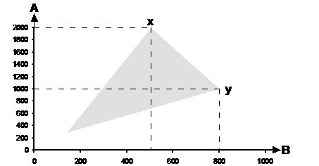
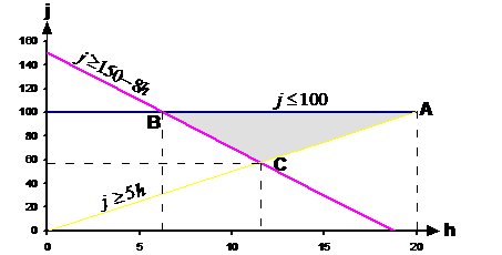
Here we have a company selling two products, product A and B. The graph shows the feasible region after all the constraints inequations have been plotted. The objective function for the profit in dollars is:
![]()
Now, obviously in general, the more of A and B that is sold the more profit the company makes. This suggests that point x or point y on the graph, or somewhere on the line in between might be the maximum profit point. The profit for the two points can be calculated:
Point x:
![]()
Point y:
![]()
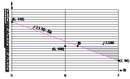
Now because the objective function (the function telling us
how to work out profit) is linear, if you travel along any straight
line in the graph, the profit will vary linearly. This tells us that if
we travel along the line between ‘y’ and ‘x’, the profit will vary linearly
from 170,000 down to 120,000. So the maximum profit point is at point ‘y’. If
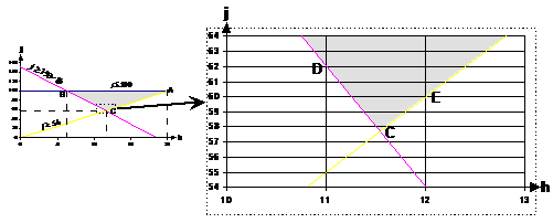
the objective function was not linear, say it was ![]() , then profit would not
vary linearly along any straight line on the graph.
, then profit would not
vary linearly along any straight line on the graph.
Notice how much more the profit is at point ‘y’ than at point ‘x’ – almost one and a half times as much. You can realise why this is by looking at the profit function – the company earns a whole lot more profit per product B sold than per product A sold. This means that any movement to the right on the graph will result in a huge increase in profit, as it represents increasing the number of product B sold. Even if the number of product A decreases, as it does travelling along the line from ‘x’ to ‘y’, it doesn’t make much difference because the profit from ‘B’ is so dominant.
|
Aircraft carriers carry large numbers of fighter jets and other aircraft on them. The Enterprising carrier is leaving port and the big wigs are trying to decide how many fighter jets and how many helicopters to put on board. They want to minimise the weight of aircraft. Each plane weighs 12 tonnes, and each helicopter weighs 40 tonnes (they’re big helicopters!). The local airbase only has a maximum of 100 fighter jets ready to go. Also, because of the supplies of fuel on board (they take different fuel), they can have no more than 1 helicopter on board for every 5 fighter jets. Some new pilots are being trained using the helicopters. The jets can be used to train only one person each, but the helicopters can be used to train 8 people. The big wigs want at least 150 people trained on this trip. How many fighter jets and helicopters should there be on board? |
|
Solution |
|
So what’s the objective of the question? Well, we’re looking for something that needs to be maximised or minimised. For this question, the total weight of all the aircraft needs to be minimised. So the objective is: Minimise total aircraft weight So what are the variables in this question – what are the things we can change the number of? Well, we have jets and we have helicopters. We’re trying to work out how many of each we need. So these are the variables. Let’s use ‘j’ to represent the jets and ‘h’ to represent the helicopters. Now, we have an objective, but we don’t have an objective function yet. This is the thing that tells us how the total weight is calculated. We can write one because the question tells us how much each aircraft weighs. We just need to use ‘j’ and ‘h’, and ‘W’ for weight: So this is the objective function we want to minimise. We need to find the constraints of the question – information that tells us limits on the variables – in this case the number of jets or helicopters. First up, we’re told that the local base only has 100 jet fighters ready to go – so that’s a maximum limit. We can write an inequation showing this information: Next piece of information tells us about the fuel situation – we can’t have more than 1 helicopter per 5 jets on the aircraft carrier. We can reword this – we must have at least five times as many jets as helicopters on the carrier. The inequation for this is: The last piece of information regards training – they want at least 150 people trained this trip. Each helicopter can train 8 people, but the jets can only train 1 person each. So if we stick an ‘8’ in front of ‘h’, we’ll have an expression for how many people are trained by the helicopters: We only need to stick a ‘1’ in front of the ‘j’ to get an expression for how many people are trained by the jets: Add these two together, and we get the total number of people trained: And we want at least 150 people trained, so this total number has to be larger than or equal to 150: So we have three constraints: We’ve got constraints, we’ve got an objective function –
we can go and plot a graph. The axes of the graph will be the two variables
– ‘j’ and ‘h’. I’m going to use ‘h’ as the horizontal axis and ‘j’ as the
vertical axis. Now, the first two constraints, Now I can go ahead and plot the graph:
Notice the three lines showing each of the three constraints. The feasible region is shaded – points inside this area satisfy all three constraints. We’re looking for the minimum total weight of aircraft on the carrier. Now, obviously, the less aircraft we have, the smaller the total weight. This means that we can rule out point A straightaway. Why? Well point B has the same number of jets as point A, but less helicopters. Point C has less jets and less helicopters than point A. So points B and C are always going to have a smaller total weight than point A. So what about points B and C? Well, point B has less helicopters but more jets than point C. This isn’t enough to tell us which point is better – we’re going to have to crunch some numbers. To do this, we need to know exactly how many jets and how many helicopters each point has. Point B has 100 jets, but how many helicopters? It looks
like about 6 on the graph, but we can use simultaneous equations to solve for
exactly how many. Now, the Now, obviously we can’t have ‘0.25’ of a helicopter, so we’re going to have to find the nearest integer number. However, we can’t use ‘6’ because it would be just to the left of the feasible area. So point B itself isn’t a candidate point. We can find the nearest point to B within the feasible zone with an integer number of jets and helicopters by drawing a zoomed in section of graph around that point:
In this zoomed in graph, I’ve drawn gridlines to show where the integer number of jets and aircraft are. The intersections where gridlines cross over each other are points which represent a whole number of jets and helicopters. Notice how point B isn’t on top of an intersection. The nearest point to B with a whole number of jets and helicopters is at (6, 100), but that point is outside the feasible zone so we can’t use it. From the zoomed in graph we can see that the best point within the feasible zone (in terms of the minimum total weight) and near to B is the point (7, 94). Other close points in the feasible zone are (7, 95), (7, 96), (7, 97) etc. but they all have more jets than (7, 94) and so represent a heavier total weight. So the best valid point near B is: Point B: j = 94, h = 7 For point C, we know it’s the intersection point where Substitute j = 5h into the second equation: And use this in the ‘j = 5h’ equation to work out what ‘j’ is equal to: Once again, we’ve got fractional amounts of aircraft! We need to find the best point near point C which has a whole number of jets and helicopters, and is still within the feasible area. Now, looking at where point C is located, ‘j’ is going to have to be rounded up, since it can’t get any smaller without going out of the feasible region. So let’s use ‘j = 58’. As far as ‘h’ is concerned – let’s check if we can round it down to 11, by seeing whether it still satisfies the constraint equations: First check h = 11 for And then check So h = 11 does not satisfy both constraints in
that region. We can try h = 12. First let’s check for Bugger. So that point doesn’t work either. We’re not getting anywhere quick trying to find an integer number of jets and helicopters near point C. We can do is plot a zoomed in part of the graph again, and find the nearest point that way:
There are two valid points near point C, point D and point E. We’ll have to compare both of these points to the best point we found near point B. Point B: h = 7, j = 94 Point D: h = 11, j = 62 Point E: h = 12, j = 60 Looks like point D represents the best combination of jets and helicopters, satisfying the training, fuelling, and jet number constraints, as well as giving the lowest total weight – 1184 tonnes. |