Linear programming

Linear programming is a technique used by manufacturers or shops to maximise profit and minimise costs.  For instance using linear programming a company can work out how many of product A and how many of product B they need to make to get the biggest profit. 

So what does linear programming look like?  Well, the ‘linear’ part gives away part of it – it involves linear equations or inequations.  To give a really simple version of it, linear programming involves plotting a few equations or inequations on the same graph, and then finding points on that graph. 

Usually, you have an equation or function which has the thing you’re trying to maximise or minimise in it.  For instance, you might be trying to maximise profit.  This is your goal or objective.

Once you’ve worked out the objective, you need to work out what affects it.  In the case of maximising profit, you need to work out how the profit is calculated.  You’re looking for an equation that has profit in it, something like this perhaps:

                                                     

Usually ‘p’ is used to represent profit.  Other variables are used to represent the number of products or items – in this case ‘A’ might represent the number of apples sold, ‘B’ might represent the number of bananas.  This is called your objective function – a function/equation that shows how your goal value is calculated.  This equation might represent something like “for every apple sold you get 20 cents profit and for every banana sold you get 40 cents profit.”

 There are also usually constraints to your problem.  For instance, a farm might not be able to grow more than 1000 apples per year, or more than 2000 bananas.  There might also be another constraint like the farm can only grown 2500 fruit in total each year.  These constraints are usually written as inequations:

                                                      

These three equations represent the three constraints described in the last paragraph.

So once you’ve got your objective function and your constraint equations or inequations, you can plot a graph.  Now, what goes on the axes of this graph?  Well, we have three variables – ‘A’, ‘B’ and ‘P’.  In linear programming, the graph shows the constraints of the problem.  Look at the three constraint equations – they only have variables ‘A’ and ‘B’ in them.  We use each of these variables for the axes.  Which one you use for which axis doesn’t really matter.

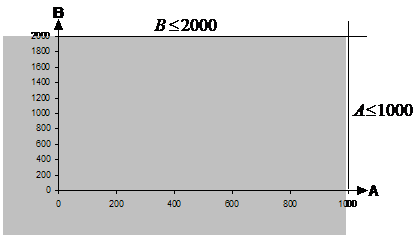
The graph needs to be plotted just like you normally plot equations and inequations.  The first two constraints are easy to plot – they’re just straight lines. The graph so far would look something like this:

The shaded area shows the region which satisfies both constraints.  Now, we need to modify the third constraint a bit in order to be able to plot it.  Since we have ‘A’ on the x-axis, and ‘B’ on the y-axis, we need to rearrange the constraint so it’s in the form “B = something…”:

                                                   

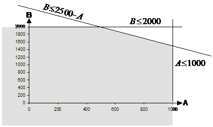
Now this is in a form we can plot.  When A = 0, B is going to be smaller than or equal to 2500.  When A = 200, B is going to be smaller than or equal to 2300, and so on.  With this line added to the graph, the shaded area changes:

This new constraint line has reduced the area of the graph which satisfies all three constraint equations.  This shaded area is called the feasible region.  Now that we’ve plotted all the constraint equations, we can get on with finding the way to maximise profit.

Somewhere within the shaded area of this graph is a point that represents the combination of apples and bananas which gives the biggest profit.  Now, we don’t need to look at any of the area which is below the A-axis or to the left of the B-axis – these parts represent selling a negative number of apples or bananas which isn’t possible.

We also don’t have to worry about looking at points such as the one on the A-axis near the 1000 mark.  This point represents selling 1000 apples and 0 bananas.  This is not going to be a maximum profit point, because we can easily just go vertically upwards, staying at 1000 apples sold, but increasing the number of bananas sold above 0.  By going upwards, we’re not reducing the profit made from apples at all, but we are increasing the profit made from bananas, so we’re increasing our overall profit.

Same with the point on the B-axis near the 2000.  This represents selling 2000 bananas and 0 apples.  We could easily slide to the right, keeping the number of bananas sold at 2000, and increasing the number of apples sold.

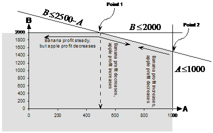
This means the maximum profit point is going to be somewhere along the top of the shaded area.  In fact, using common sense we can work out that the maximum profit point is either going to be at point 1 or 2:

If you go to the left from point 1, you reduce the number of apples you sell and hence your overall profit goes down.  If you go right and down from this point, you reduce the number of bananas but increase the number of apples you sell, so your overall profit might go up or down. At point 2, going left and upwards increases the number of bananas you sell, but decreases the number of apples sold. You can’t go right from point 2, only down, which would result in a decrease in the number of bananas and hence overall profit.

Once you’ve found your candidate maximum profit points, you need to work out how many of each item is sold at each point. You can read these off the graph – at point 1 it’s 2000 bananas and about 500 apples. At point 2, it’s about 1500 bananas and 1000 apples. To find out which point is more profitable, you can calculate the profits at the two points using the original objective function. We’ll need exact values of A and B at the two points to put into the objective function.

At point 1 we can read the value of B off the graph exactly because it’s right up against the  constraint line, so we know B is 2000. However, reading the value of A off the graph, we have to estimate where point 1 lines up with the A-axis. We can work out the exact value of A by using the constraint equations.  Since we know B accurately, we need an equation which has A in it as well.  The constraint inequation  has both A and B in it.  The equation for just the line, not the line and area beneath it, is .  Since this line passes through the maximum profit point, we can use it to work out what A is:

                                                    

We can do the same to work out the value of B at point 2. Since point 2 is right up against the  constraint line, we already know A is exactly 1000.

                                                    

Now that we have the exact values of A and B for each point, we can work out which has the greater profit:

Point 1

Point 2

From this comparison we can see that point 1 is the most profitable.