Solving them algebraically

There are some situations when you will be given two simultaneous equations, and one or both of them will be quadratic equations.  For instance, you might be given these two equations:

                                                       ................................................. (1)

                                                          .................................................... (2)

The first equation is a quadratic equation.  The second is just a linear one.  To solve these simultaneous equations, what we are looking for are (x, y) values that make sense in both equations.  For instance, take the point x = 3, y = 15.  These two values make sense in the second equation, but not in the first one.  So these two values aren’t a solution to the simultaneous equations.

What we can do is equate the two equations.  We’re looking for values of ‘x’ and ‘y’ that work in both equations.  So what we can do is say something like, “Let’s assume that the values of ‘y’ are the same in each equation.”  If the ‘y’s are the same, then we can do this:

                                                  

What I’ve done is say that what ‘y’ is in the first equation is equal to what ‘y’ is in the second equation.  Now, we’ve only got ‘x’s left in this equation, so let’s try and solve for the value of ‘x’.  We can do this by rearranging the equation so all the terms are on one side:

                                                

Now we’ve got a quadratic equation.  We can use the quadratic formula to solve for the possible values of ‘x’.  Now, the equation is already in the standard quadratic equation form:

                                                     

This means that the values of ‘a’, ‘b’ and ‘c’ are:

                                                

So we can use our quadratic formula to work out the possible values of ‘x’:

                                        

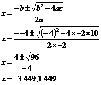
These are our ‘x’ values, to work out the ‘y’ values we just need to substitute these ‘x’ values into one of the original equations.  It’s generally better to use the simpler equation in this situation, to help keep it as easy and quick as possible.  This means I’m going to use the 2^nd equation:

                                       

So the two solutions to this set of simultaneous equations are:

                                        

Solving them using a graph

The other option you have for solving the simultaneous equations is to plot a graph showing both functions:

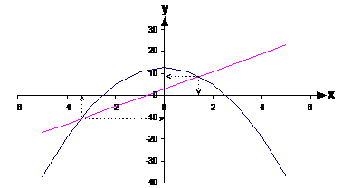
This method isn’t as accurate, but can be quicker, or easier if the equations are very complicated.  The solutions to the simultaneous equations are represented by the intersection points of the two lines.  By reading the x-y coordinates off the graph you could give an answer like this:

                                               

We can’t give as many significant figures in our answers because reading off the graph is only approximate.  These answers are pretty close though to the algebraic answers.

Milk lover question

Jeremy is a milk lover.  He buys his milk in square based prism one litre containers.  He drinks the milk out of a huge cylindrical glass he keeps especially for drinking milk – no other liquid is allowed!  One litre of milk fits perfectly into his glass, which is the same height as the 1 litre carton.  One day the shops advertise that they have new 2 litre, 3 litre and 4 litre cartons, with base side lengths of 8.944 cm, 10.95 cm and 12.65 cm.  These new cartons all have the same height as his glass.  He wonders how much wider the diameter of his glass would have to be to fit these amounts.  Derive the formula relating the diameter of a glass to the base side length of the carton, and use it to work out the required glass diameter for the new carton sizes.

Solution

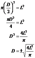
So he’s got a cylindrical glass he wants to be able to fit certain amounts of fluid in.  The question asks us a very specific thing – we need to derive (come up with) an equation that tells us how big (in terms of the diameter) a glass has to be to fit all the milk from a carton with a certain base side length.  The question also tells us that the heights of the cartons are the same as the glass.  So what we can do is write down a few volume formulas straightaway, one for each item:                                                                                                             Now, our requirement is that the volumes of the carton and glass be the same.  See where we’re heading?  We’ve got two equations, and we know that the ‘V’ in each one is the same.  So we can equate the two equations and get this:                                                     The question has told us that the height of the glass and cartons are the same, this means that:                                                         This means we can cancel out the two ‘h’s on either side of the equation:                                                                                                               We want a formula that gives us the diameter of the glass for a certain base side length of the carton.  Currently we’ve only got the radius in the formula, we can substitute in ‘D/2’ for ‘r’, since the radius is half the diameter:                                                     Now we can use this equation to work out the required glass diameters for the new carton sizes. Note that we only use the ‘+’ answers, since the ‘–’ answers don’t make sense in this situation.   Carton size Required glass diameter     2 L 10.09 cm     3 L 12.36 cm     4 L 14.27 cm

 

Modelling car acceleration using quadratics

Ok, so here’s the moment for all you revheads out there – let’s talk about car accelerations.  0 – 100 km/hr times!  0 – 200 km/hr times!  400 metre drag times!

Of course there’s always a mathematical catch.  In this case, we’re going to try and model the speed of a car as it accelerates by using a quadratic model.  When a car accelerates from a stopped position, its speed increases.  The speed keeps getting faster as time goes by.  One of the important statistics that are often quoted about sports cars is their time to do 0 – 100 km/hr.  So there are two variables here – time and speed.

Now the speed the car is moving at when the accelerator pedal is floored (pressed all the way down) depends on how much time has gone by.  The car obviously will be at a higher speed after 4 seconds then after 2.  So there is a relationship between time and speed.  This relationship for cars can usually be modelled approximately by a quadratic relationship.  So let’s look at some data:

This data is typical of a fairly high end sports car, such as a Porsche.  One thing to note is that often car’s times are expressed for 0 – 60 miles per hour.  This is very similar though to 0 – 100 km per hour, since 60 miles per hour equals about 97 km per hour.  Before you try and fit any models it’s usually a good idea to plot the data to get a feel for what you’re dealing with.  How to plot the data?  Well when the table says that it takes 1.7 seconds to get from 0 to 60 km/hr, you can read this as the car is going 60 km/hr after 1.7 seconds:

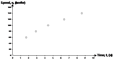
Now you could try and fit a linear model to this data, but it looks like a quadratic curve would fit it more nicely.  But if we did try and fit a quadratic curve through it, we might get something like this:

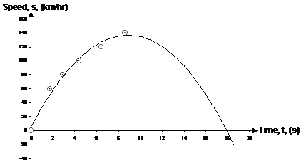
This graph is telling us that with the accelerator fully pressed, the car is only going to reach about 140 km/hr, before, with the accelerator still fully pressed, it starts to slow down!  This doesn’t really make sense, especially for a sports car which we know can get well over 200 km/hr.  It turns out that you can form a much better quadratic model if you have speed as the independent variable on the x-axis, and time as the dependent variable on the y-axis, like this:

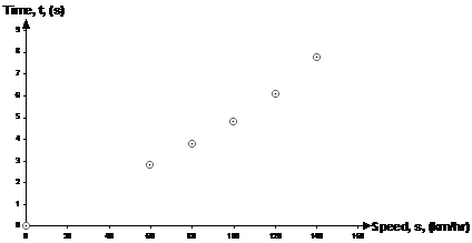
Because the data passes through the origin exactly (when the car is just about to start at 0 seconds it’s got a speed of 0 km / hr), there is no ‘c’ term in the general form of the quadratic equation.  Also, remember that ‘s’ is the ‘x’ type variable, and ‘t’ is the ‘y’ type variable:

                                                    

One more simplifying assumption that can work well in this case is to ditch the ‘bs’ term, and just assume that a  relationship can describe the data well enough.  What often happens is you pick one data point (say the end one), and use it to work out the value of the ‘a’ in the relationship.  So if we use our end data point, we get:

                                                    

So:

                                                    

If you plot a line on the graph using this equation, you get quite a close fit to the original data:

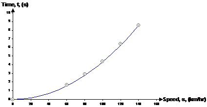
This quadratic model makes much more sense than when we had the variables around the other way.  Now, as the car gets faster, it takes longer to increase the speed, represented by the increasing slope as you move to the right on the graph.  This is plausible – as the car gets to higher speeds the amount of ‘oomph’ it has left to accelerate decreases, so the speed goes up more slowly.  It’s slightly unrealistic in that it predicts the car can accelerate forever, given enough time, but most models are only useful/realistic within a range of values. We just need to remember that even though our relationship predicts that after 438.8 seconds the car will be at 1000 km/hr, this is outside the limits of our model and hence cannot be used.

Usually now questions will ask you to use your formula to predict various values, such as:

Car acceleration question

How long for the car to reach 200 km/hr? After 15 seconds how fast will the car be going? After 30 seconds, how fast will the car be going? Comment on the accuracy.

Solution

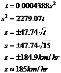
The first part’s easy – just plug 200 km/hr into your relationship:                                                  The second part’s pretty easy too; rearrange the relationship, and then just plug in numbers:                                                    You should explain why you took only the positive answer (the negative answer makes mathematical but not physical sense). The last part is easy too, you repeat the process we just did, but for 30 seconds:                                                     The ‘comment about the accuracy’ part is asking for one of those answers where you talk about how we have a model, but that the model is only valid for a limited range of times and speeds.  Our data that we made the model from only goes to 10 seconds, yet we’ve just tried to predict a speed after 30 seconds using this model.  This is rather severe extrapolation (estimating values outside the data you’ve been given), so it’s probably not very valid to use our model for a time so far outside the data we’ve been given.